Big O Notation Time and Space Complexity
A note for those who feel lost with Big O: If Big O feels too complex at the moment, you shouldn't let this block you from studying for interviews, especially if you are looking for your first job. If you focus on writing clean, well-structured code and practice learning the intuition to solve data structure and algorithm interview questions, you'll still set yourself up to succeed in many interviews. Not learning Big O may disqualify from a subset of companies, but there are still many job opportunities available at companies that don't ask about this concept.
Big O measures how long an algorithm takes to run.
We're going to fully understand Big O, but let's first define it without all the math before we dive in.
We measure the speed of an algorithm based on the approximate number of steps that it takes to run. I say "approximate" because Big O is actually meant to be simple and provide a high-level explanation. With Big O, we ignore the line-by-line details of the code and don't care about every single calculation.
We calculate Big O relative to the size of the input which we denote by n.
So if we are given an array, array.length == n.
We use the letter n because we're just saying we want to know approximately how many operations the algorithm would require for any array.length.
If we iterate through the array once with a for loop, we touch every item — or all n items.
With this single loop, we say that for the input array length n, our function takes O(n) operations.
We don't care about any of the other calculations happening inside the for loop.
Big O can be an intimidating topic, especially for new developers. This lesson will break it down and walk you through it step-by-step to make sure you feel completely comfortable with Big O's concepts and how to apply them to a programming interview.
How Candidates are Graded for Hiring
To understand why we need Big O, we first need to understand how candidates are graded in their coding interviews.
Determining if someone will be hired is essentially based on 3 general metrics:
- Experience (work background or personal projects)
- Soft skills (will you be a good teammate and enthusiastic about the product)
- Code (can you solve problems effectively)
Experience and soft skills are aspects you can work on, but for now we will look closer at how coding is measured. Being able to solve the problem is obviously important. However, what you are actually judged on in an interview is how good the code is that you write to solve the problem.
Code will be judged by two factors:
- Scalable (objective)
- Readable (subjective)
When we talk about scalability, we are referring to the Big O complexity of an algorithm and the number of operations it will take to run.
The reason we put so much effort into Big O is that it's objective and can be taught academically. This means that if two algorithms solve the same interview question but have different Big O complexities, we can say the one with the better Big O is the better solution (in terms of scalability).
For example, if we have two algorithms that solve a problem at O(n) and O(n2),
we can objectively say that the O(n) is better because we know it will require fewer operations.
The O(n) solution would touch each item in the input for a total of n times, and the O(n2) solution will touch the input items n x n times.
input size    |         Operations
     n        |      O(n)        O(n^2)
------------------------------------------
     1        |      1           1
     2        |      2           4
     3        |      3           9
    ...       |
    100       |      100         10000
    ...       |
    1000      |      1000        1000000
    ...       |
     n        |      n           n^2
Readable code, while equally important, can encompass many traits. Your interviewer's opinion is ultimately the judge of your code readability. As you work through this course, you will learn to write better code. This comes with practice and repetition to understand what clean code looks like and is not as easily taught in a single lesson.
Advice if Big O is New to You
If this concept is new and intimidating to you, my biggest piece of advice is to try not to overthink it. Big O is a general and high-level representation of an algorithm. You are not expected to analyze a program line-by-line and account for every single operation.
What you do is find the block of code in the algorithm that requires the most iterations through the input data structure. Then all you need is an understanding of the approximate time complexity for common scenarios — O(n) for single loops, O(n2) for nested loops, O(n log n) for sorting, etc.
As long as you can recognize and locate the most expensive block of code based on these general rules, you will have figured out 90%+ of what you need to know about Big O for interviews, and the remaining 10% you will gain through experience as you work through the course.
What Big O Means
Big O determines how an algorithm scales.
Another way of saying this — Big O judges how fast our algorithm handles a very large number of items.
- We judge speed based on the number of steps and not calculated time (ie. seconds or minutes).
- We only care about the steps that increase based on the input size.
nisn't an exact number. It just means when the input gets "very large". For me, I just imaginen = 1000000to put it in real terms. It's large enough to be significant but not so large you get lost in all the 0's.
In production software, our code may need to handle millions or even billions of items. We need to make sure our algorithm stays fast as the amount of data it needs to handle grows.
As the amount of data increases, the difference between a good and bad solution becomes more exaggerated. Bad solutions tend to get even worse relative to a good solution as you add more data.
So how does Big O actually determine this?
Let's do a thought experiment. Say we have the following functions:
If they are given the same input, how will we know which one takes more time to run?
- What if the input size
nis just 1 item? - What if the input size
nis 1,000,000 items? - What if #2 is executed on your cell phone and #3 is executed on a super computer?
- What if we execute #2 locally and #3 by calling an API on a remote server?
If we try to time which algorithm is faster, it is entirely dependent on the environment and amount of data.
For n = 1 item in the input, they will all finish nearly instantaneously.
However, if we ran the functions on the same computer for 1,000,000 items, #1 will still finish instantly, and then #2 will finish much faster than #3.
#1 has no dependence on the input. No matter the data size, it will always perform the same number of operations, so we call this constant time O(1).
It performs the same number of operations each time because the loop always goes from 0 to 20, regardless of the value used for input.
Since #2 uses one for loop, it will iterate the input for all 1,000,000 items once, and this is what we call O(n).
#3 has nested for loops, so it will iterate the input 1,000,000 times for all the 1,000,000 elements
for a total of 1,000,000,000,000, and this makes it an O(n2) algorithm.
That is 1 million vs. 1 trillion operations for #2 vs. #3.
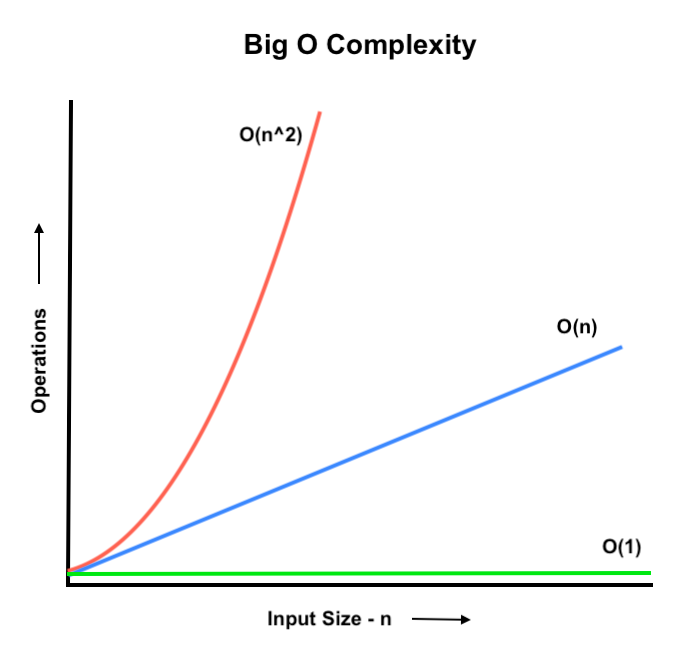
If we graph the time complexities, we can see that the O(n2) separates from the O(n) and the operations get drastically larger for a given input size. The O(1) stays flat and doesn't change with input size.
This is why we care about scalability and how a solution grows with input size. We can judge how a solution will perform with concrete metrics and irrespective of the environment that the code is executed in. When the input size is large, the number of required operations blows up for the slower algorithm.
Although this won't be asked in interviews, let's see how the varying Big O complexities would approximately translate to the time required to complete an algorithm when we normalize an O(n) operation with 1 billion items to take 1 second. In our thought experiment, the time difference O(n) and O(n2) at 1 million items would be 1ms vs. 16.7 minutes. That's the difference between blazing fast and "broken" from a user's perspective.
| Input size | log n | n | n log n | n2 | 2n | n! |
|---|---|---|---|---|---|---|
| 10 | 0.003ns | 0.01ns | 0.033ns | 0.1ns | 1ns | 3.65ms |
| 20 | 0.004ns | 0.02ns | 0.086ns | 0.4ns | 1ms | 77years |
| 30 | 0.005ns | 0.03ns | 0.147ns | 0.9ns | 1sec | 8.4x10¹⁵years |
| 40 | 0.005ns | 0.04ns | 0.213ns | 1.6ns | 18.3min | -- |
| 50 | 0.006ns | 0.05ns | 0.282ns | 2.5ns | 13days | -- |
| 100 | 0.07 | 0.1ns | 0.644ns | 0.10ns | 4x10¹³years | -- |
| 1,000 | 0.010ns | 1.00ns | 9.966ns | 1ms | -- | -- |
| 10,000 | 0.013ns | 10ns | 130ns | 100ms | -- | -- |
| 100,000 | 0.017ns | 0.10ms | 1.67ms | 10sec | -- | -- |
| 1'000,000 | 0.020ns | 1ms | 19.93ms | 16.7min | -- | -- |
| 10'000,000 | 0.023ns | 0.01sec | 0.23ms | 1.16days | -- | -- |
| 100'000,000 | 0.027ns | 0.10sec | 2.66sec | 115.7days | -- | -- |
| 1,000'000,000 | 0.030ns | 1sec | 29.90sec | 31.7years | -- | -- |
4 Steps to Calculate Big O
We explored that Big O means we want to understand how the number of operations required by an algorithm increases as the input size gets very large. Let's see how we can use this knowledge practically to be able to calculate the Big O of an algorithm.
There are 4 steps we follow:
- Worst case
- Drop constants
- Drop less significant terms
- Account for all input
Step 1. Worst case
When we're calculating the Big O time complexity of an algorithm, we base it off the worst case possibility.
We want our Big O to describe the tightest upper bound of our function.
Consider this simple example:
In the best case, we only iterate 1 item so we actually found the item in O(1) time — the input size didn't matter, and this is an edge case. This is a very rare scenario and doesn't provide much meaning.
In the average case, we will iterate half the items array which is O(0.5 n). (But we also drop constants which you'll see in step 2).
In the worst case, we would have to iterate the entire array to find the last item which is O(n).
Imagine this was in production, and we wanted to search in an array of 1,000,000,000 items. 25% of the time, we would expect to iterate through at least 750,000,000 items. This is still a lot of people that would have a bad experience.
Therefore, we view Big O as a bound on our problem. For our code to be reliable, we need to make sure all reasonable scenarios are within the bounds.
We say our Big O complexity is the worst case scenario which allows us to confidently account for any outcome.
Step 2. Drop constants
You may have noticed when we talk about Big O, we only refer to n and don't say things like 5n or O(2n + 3n).
We allow ourselves to ignore constants because it would require too much knowledge of what's happening in the compiler or how the system optimizes our code and converts it to machine language.
As we said earlier, Big O is meant to be simple. Trying to account for all the operations adds a ton of difficulty without really providing any new information. Take a look at the example below to see why.
So what is this Big O? You may be tempted to say the case1 function is O(3n) because we have 3 separate loops.
However, in case2 we still call our print function the same number of times.
We also have no idea how our programming language will interpret this code and execute underneath the hood.
Now let's think about what happens if we pass 1,000,000 items to all 3 functions.
We believe case1 and case2 may perform between 1 to 3 million operations.
However, case3 performs 1,000,0002 or 1,000,000,000,000 operations.
The difference between 1 and 3 million becomes insignificant when compared either to 1 trillion operations.
We allow ourselves to accept the fact that we only care about the trend of the algorithm as it scales with large input size and only compare runtimes of different order complexity, ie. O(n) vs. O(n2).
This leads to another learning outcome. Since we drop constants, back-to-back iterations through an input are all still O(n). Nested loop iterations always lead to O(n2) or worse runtimes, depending on the level of nesting. Always try to find a way to run your loops sequentially instead of nested to improve runtime.
Step 3. Drop less significant terms
In step 2, we saw that we drop constants, and when we have a sufficiently large input, the difference between n and 3n loses significance.
We can take this one step further and say that if we have operations within an algorithm that utilize different Big O time complexities, we only consider the slowest Big O. For example, if we have O(n2) and O(n) within a function, we simply say the function operates in O(n2) time.
With an input size of 1,000,000, we would have 1000000 + 1000000000000 = 1000001000000 operations.
Using our table above, that would be 16.7 minutes + 1 millisecond, which makes the millisecond meaningless.
The larger term is so overpowering that we allow ourselves to reduce the solution to simply O(n2).
Step 4. Account for all input
There are problems where we receive multiple input data structures.
If we can't make any assumptions about the size of them, we need to account for both of them when calculating our Big O complexity.
The most common syntax is to refer to one input as n items and the other input as m items.
Common Big O
Big O Visualized
These are some of the most common time complexity from fastest to slowest.
O(1) - constant time
Constant time or O(1) means that we don't iterate through our data structure. The operations that occur never increase, regardless of how our large our input gets.
Examples of constant time operations include: accessing a hash table by key, popping the last item of an array, or any normal arithmetic.
O(log n) - log time
The most common example of log time is a binary search. Log time happens when you repeatedly divide the input. You can think of this in contrast to quadratic time which multiplies the input and explodes.
The repeated division shrinks our solution so quickly that O(log n) is blazing fast, even for very large n.
O(n) - linear time
This happens where we iterate through our input data structure once (or sequentially). As long as we don't nest loops, we will operate in linear time.
If we have an input array with length 1,000,000, our for loop would iterate through one million items.
If we have an input array with length 1,000,000,000, our for loop would iterate through one billion items.
An O(n) time just means that the operations required is simply the length of the input.
The operations and input size increase 1-for-1, or linearly.
This applies to other iteration methods such as
forEach,map,filter,reduce. They all iterate through our input data structure once, just like aforloop.
O(n log n) - log-linear
This is between linear and quadratic time where you perform n x log n operations.
This is most commonly seen in sorting algorithms, and you can assume a native sort function will operate in O(n log n) time.
The reason O(n) < O(n log n) < O(n2) is that log(n) is greater than 1 and less than n.
So for O(n log n), we multiply n times a number that is 1 < log(n) < n.
O(n2) - quadratic time
This happens when we nest loops. Brute force solutions are often quadratic time and are rarely acceptable as a final answer.
The more nesting you have, the more the exponent increases. If you have three nested loops, then the complexity becomes O(n3).
The general name for when we raise n to a power is known as polynomial time.
Quadratic time means we have polynomial time where we know the exponent is 2.
Be careful with hidden quadratic time. You may think you are doing a single loop but may perform another O(n) inside it. An example of this is when you slice array which is also linear time.
O(2n) and O(n!)
The cases that are worse than O(n2) are a little more rare and specific. We'll visit these as needed in the course, but both scenarios are very bad and should be avoided at all costs.
An example of O(2n) is a brute force recursive algorithm to calculate a Fibonacci number. This is explored further in the recursion module and the dynamic programming module.
The worst complexity is O(n!), and this occurs when you calculate all the permutations of an input.
Space Complexity
Up to this point, we have been talking about how long algorithms run by describing their time complexity in terms of the number of operations. There is another factor we should consider which is space complexity. Space complexity is represented using the same notation, but it refers to the amount of additional space in memory our algorithm must use.
With the increased importance of fast software and the decreasing price in memory, time complexity has become the dominant consideration. However, we can't ignore space. Running out of memory is a real issue in software engineering, and it can cause our program to crash. Memory (the space we have available for our program to execute) is a limited resource that we need to account for.
The most common scenario to add to the space complexity of an algorithm is when we utilize an auxiliary data structure in our solution algorithm.
The way we calculate space complexity is nearly identical to time complexity.
For example, if we need fast key-value access, we can add a hash table.
We put all n items in the hash table, so it requires O(n) space.
This means we've stored n items in memory.
Amortized Time
This is an advanced topic, so ignore it for now if your head is still spinning. You will see it later in the course.
When we calculate the Big O of an algorithm, we do so by considering the worst case scenario, which is the slowest time complexity. There is an exception to this rule known as amortized time.
When we have numerous operations that occur with a fast time complexity and then on a very rare occasion have a slow operation, we actually ignore the slower operation. The fast operations overpower the slow one because they happen in nearly all the cases.
An example of this is a dynamic array that resizes and doubles its capacity each time it becomes filled.
A push to the array takes O(1) time.
If we have 1,000,000 items in the array and a capacity to hold 2,000,000, we could push 999,999 times at O(1) time
before it is resized once at O(n) time.
A simple way to think about it mathematically is that we have 1 operation that requires O(n) time.
We have n - 1 operations that use O(1) time.
Since it takes nearly n operations before our O(n) occurs again,
we say that the frequent fast operations pay for the cost of the very rare and slow operation.
Typically for Big O we like to look at the worst case we can expect per algorithm. With amortization, we consider the complexity per operationAmortizedTime since they are so unevenly distributed.